
Expression Shape
The Expression shape is the mathematical heart of every Modellus model. It is where you define equations, parameters, differential equations, recurrences, and conditional logic that drive the simulation.
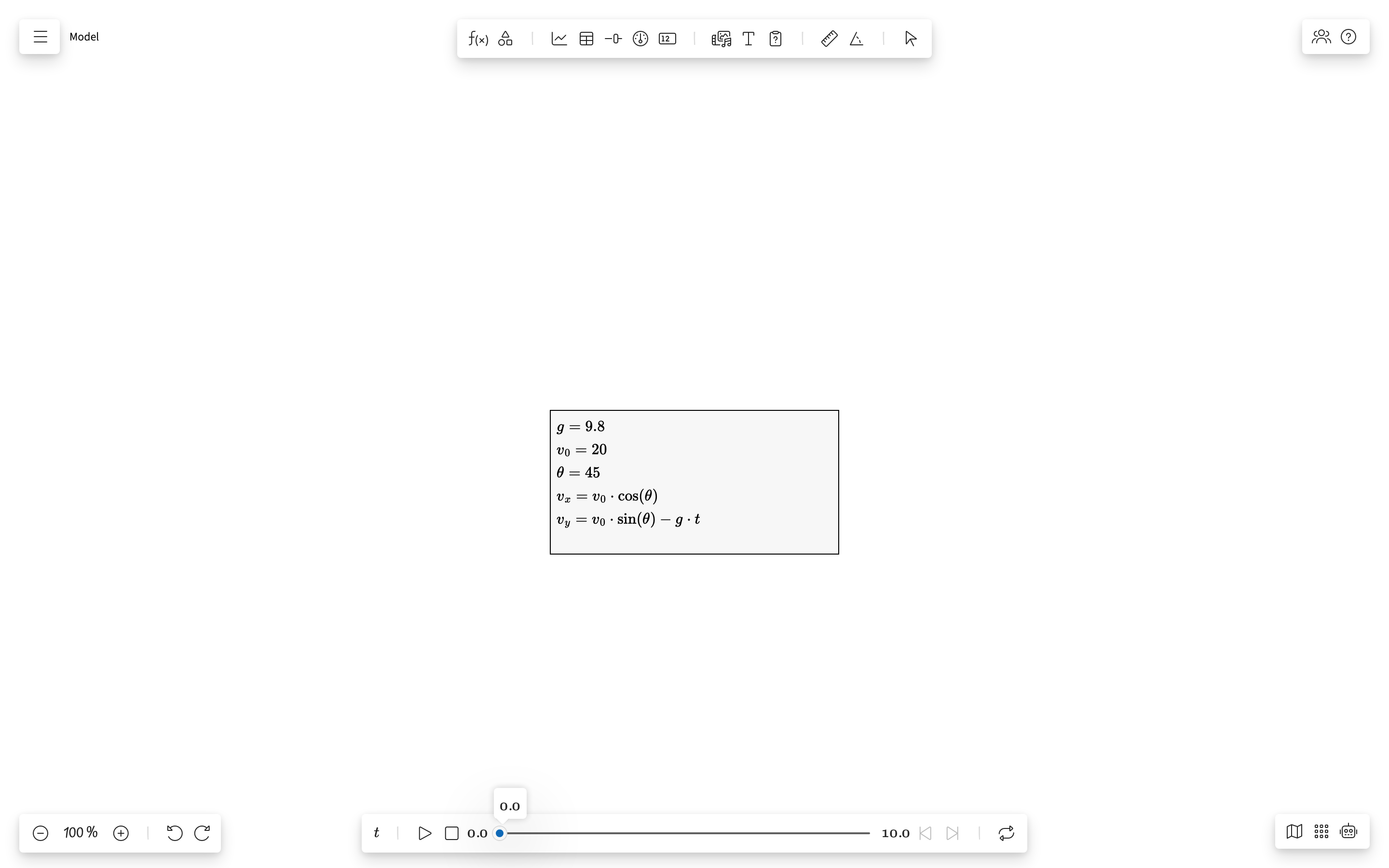
Overview
An Expression shape contains one or more mathematical statements written in LaTeX-like syntax using a MathLive math field. Each statement occupies one line. All Expression shapes in a model share a single calculator system — term names must be globally unique across shapes.
Reading an Expression
When a shape holds two or more equations, they are shown as one block sharing a single equals-sign column: the left-hand sides are right-aligned against the equals sign, the right-hand sides are left-aligned after it, and the block is centred in the card. Only the primary equals sign of each line is aligned — an equals sign inside a condition, a fraction or brackets is left where it is. A shape holding a single equation is shown as before. Alignment is presentation only: the model still stores one plain line per equation.
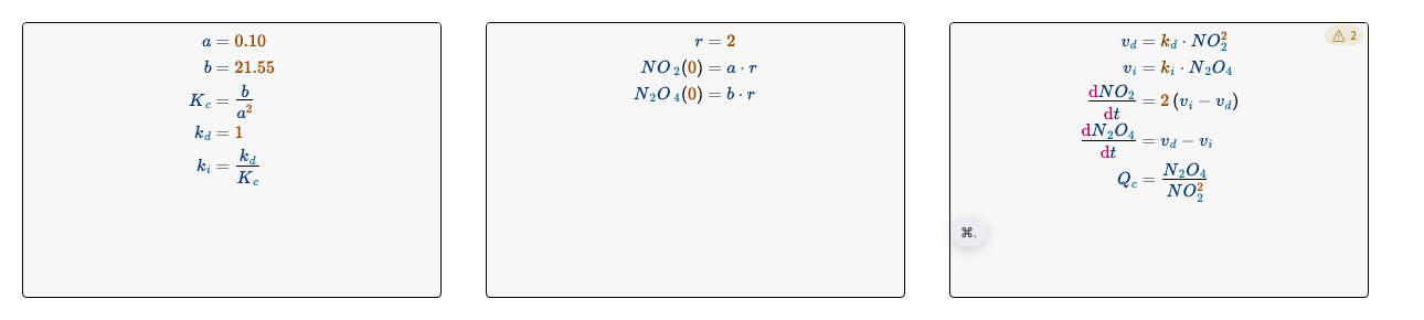
Every part of an expression is coloured by what it means:
- Variables — dark blue
- Numbers — orange
- Operators, relations and brackets — neutral grey
- Functions such as
sin,lnorsqrt— green - Derivatives — the
dofdx/dt, partial signs, primes and dot derivatives — magenta - Qualifying subscripts such as the
cofK_c— light blue - Iteration indices such as the
nofx_n— purple - The terms the model advances by — the independent term
tand the iteration termnwherever they stand on their own — purple, the colour they already carry as an index - Rows the model cannot read — red, and marked where they stand (see below)
A row the model cannot read is said so on the card itself, not hidden behind a hover. The row is written in red and carries a band across it, the card is bordered in red so it can be picked out from across the board, and a panel at the foot of the card says why, in the language the rest of the editor is written in. Where the row is missing something — a value, a bracket — a dotted slot is drawn in the row at the place it belongs, the way an unfilled slot of a template is drawn; where the missing piece is inside a fraction or a root, that fraction or root is underlined instead, since the place cannot be named more closely than the symbol holding it. A symbol that cannot stand where it was written is underlined where it stands. The panel opens whenever you reach for the card — the pointer over it, the card selected, or the caret in it — and carries the readings alone, with no heading over them and no row named in front of each one: pointing at a reading lights the row it belongs to, and clicking it puts the caret there. Rows are checked as you write rather than only when you step away, except for the row the caret is standing in: a row is half-written for as long as it is being written, so it is left alone until you leave it.
The colours name a family, not a fixed shade. Each one is read from the --math-* theme tokens and then adjusted to the card it is painted on: the hue stays, the lightness moves until the text stands clear of the background, and the colour is deepened at the same time. A card painted white gets deep, saturated colours; a card painted black or dark grey gets bright ones; changing the card colour repaints the expression at once. Every colour keeps at least the contrast the accessibility guidelines ask for, and the operators are held one step quieter than the variables. The caret and the selection highlight follow the same rule, and so does the text colour of the card, which is what draws the brackets, the fraction bars and the root signs: it is left exactly as you chose it and only lifted when the card would otherwise swallow it. None of this reaches the model: an expression saved or copied out never carries a colour.
Toolbar

The toolbar appears when you select an Expression shape. It provides:
- Color picker — Change the shape accent color
- Shortcuts picker — Quick insertion of common mathematical templates
- Delete — Remove the shape from the board
Statement Types
Each line in an Expression shape is parsed as one of these statement types:
| Type | Syntax | Example | Description |
|---|---|---|---|
| Parameter | name = value |
g = 9.8 |
A constant value. No dependency on other terms or the independent variable. |
| Function | name = expression |
E = ½·m·v² |
A computed value depending on other terms or the independent variable. |
| Differential | dx/dt = expression |
dx/dt = v |
First-order ODE. Requires an initial value in shape properties. |
| Recurrence | x_{n} = expression |
x_{n} = x_{n-1} + v·Δt |
Iterative step definition. Subscript determines step offset. |
| Conditional | name = \begin{cases}...\end{cases} |
v = { 0 & t=0 \\ a·t & otherwise } |
Piecewise definition. At least two branches required. |
| Function with argument | f(t) = expression |
h(t) = v₀·t - ½·g·t² |
Explicit argument notation (cosmetic; behavior same as Function). |
| Display | expression |
F = ma |
Visual label only. Not computed by the calculator. |
Arithmetic Operators
| Operator | LaTeX | Keystroke | Description |
|---|---|---|---|
| Addition | + | + | Sum of two expressions |
| Subtraction | - | - | Difference of two expressions |
| Multiplication | \cdot | * | Explicit multiplication (· symbol) |
| Implicit multiplication | 2x | 2x | Coefficient followed by name or parenthesis |
| Inline division | / | / | a/b inline notation |
| Fraction | \frac{a}{b} | / (in numerator position) | Display-quality vertical fraction |
| Power | ^{n} | ^ | Exponentiation |
| Factorial | x! | ! | Postfix factorial for non-negative integers |
| Square root | \sqrt{x} | \sqrt | Square root |
| Negation | -x | - | Unary negation |
Factorial note: Factorial uses postfix notation (n!) and is intended for non-negative integer values.
Comparison Operators
Used in conditional (\begin{cases}) branches:
| Operator | LaTeX | Meaning |
|---|---|---|
| = | = | Equal to |
| > | > | Greater than |
| < | < | Less than |
| ≥ | \ge or \geq | Greater than or equal |
| ≤ | \le or \leq | Less than or equal |
| ≠ | \neq | Not equal to |
Conditions can be chained (e.g., 0 < x < 1) or combined with \lor (OR) and \land (AND). The \text{otherwise} keyword acts as an else branch.
Built-in Functions
| Category | Function | LaTeX | Arguments |
|---|---|---|---|
| Trigonometric | Sine | \sin\left(x\right) | 1 |
| Cosine | \cos\left(x\right) | 1 | |
| Tangent | \tan\left(x\right) | 1 | |
| Cotangent | \cot\left(x\right) | 1 | |
| Secant | \sec\left(x\right) | 1 | |
| Cosecant | \csc\left(x\right) | 1 | |
| Inverse Trig | Arc sine | \arcsin\left(x\right) | 1 |
| Arc cosine | \arccos\left(x\right) | 1 | |
| Arc tangent | \arctan\left(x\right) | 1 | |
| Hyperbolic | Hyperbolic sine | \sinh\left(x\right) | 1 |
| Hyperbolic cosine | \cosh\left(x\right) | 1 | |
| Hyperbolic tangent | \tanh\left(x\right) | 1 | |
| Logarithmic | Natural log | \ln\left(x\right) | 1 |
| Logarithm base 10 | \log\left(x\right) | 1 | |
| Two-argument | Maximum | \max\left(a, b\right) | 2 |
| Minimum | \min\left(a, b\right) | 2 | |
| Modulo | \mod\left(a, b\right) | 2 | |
| Utility | Sign | sign\left(x\right) | 1 — returns -1, 0, or 1 |
| Random | rnd\left(x\right) | 1 — random float in [0, x] | |
| Integer random | irnd\left(x\right) | 1 — random integer in [0, x] | |
| Integer part | int\left(x\right) | 1 — truncate to integer | |
| Round | round\left(x\right) | 1 — round to nearest integer | |
| Other | Determinant | \det\left(x\right) | 1 |
\left( and \right) delimiters. Bare parentheses are not valid in function calls. The math field inserts these automatically.
Constants
| Name | LaTeX | Value |
|---|---|---|
| Pi | \pi | 3.14159… |
| Euler's number | e or \E | 2.71828… |
g is not a built-in constant. Define it as a parameter: g = 9.8.
Special Syntax
Finite Difference (Δ)
| Syntax | Meaning |
|---|---|
\Delta x | x(current) − x(previous). For the independent variable: the step size. |
\Delta\left(expr\right) | Finite difference applied to a sub-expression. |
Subscripts (Step References)
| Syntax | Meaning |
|---|---|
x_{n-1} | Value of x from the previous iteration |
x_{n} | Current iteration (LHS of recurrence) |
x_0 | Initial value of x (bare digit, no braces) |
x_{0} | Initial value (braces form) |
Indexed Terms (Element References)
A term can stand for many values at once — the oscillators of a wave, say — by being defined over an element index instead of over time. The index is bound by the assignment, so it never becomes a variable of the model:
y\left[i\right] = A\cdot\cos\left(k\cdot i - \omega\cdot t\right)| Syntax | Meaning |
|---|---|
y\left[i\right] = … | Defines y over element indices; the body is evaluated once per element asked for |
y\left[3\right] | Element 3 of y |
y\left[i\right] | Element i, where i is any expression |
s = y + z | Superposition: s is indexed too, added element by element |
This is a third index space beside the two above: y_3 reads y at iteration 3 and y\left(3\right) reads it at independent value 3, while only the square brackets read an element. An indexed term holds no single value, so it is read for its elements rather than shown as a number.
An Oscilloscope object reads them: name the indexed terms in its Waves and each is drawn across its graticule, one trace per row. Two travelling waves added this way — one with -\omega\cdot t, one with +\omega\cdot t — give a standing wave with fixed nodes. A Piano publishes one: the chord it is holding, one element per sample.
A Mechanical wave object works from a plain term instead. Name one the model works out for itself — y=A\cdot\sin\left(\omega\cdot t\right) — in its Wave row and the chain repeats what that term has been doing: every iteration hands the first oscillator the value the term has just taken and moves the one before it along, so the chain holds the last values of the run, oldest at the far end, and the motion travels down it as the run goes. It holds one value per oscillator, so Samples is also how far back it reaches. Write a name the model does not define and the object goes the other way: it works its wave out from its amplitude, frequency, speed and phase and hands the model what its reference oscillator is doing under that name. The name becomes a term of the model — it is in every list of terms, the way a name the model assigns is — so it can be graphed against time, read in a definition (z=2\cdot y) and added to another object's reading (s=forward+back). A name the model does define is the model's own — an assignment, over time or over element indices, is read rather than written over — and an object taken off the board takes its term with it.
Units Annotation
Append display-only units after any statement:
v = 10 \quad\textcolor{gray}{\mathrm{m/s}}Units are cosmetic — the engine does not validate or convert them.
Dotted Names (Child References)
Reference terms from child shapes inside a Referential: body.x, particle.velocity.
Keyboard Shortcuts
The MathLive math field supports these keyboard shortcuts for fast input:
| Action | Shortcut | Result |
|---|---|---|
| Open template palette | ⌘. (macOS) · Ctrl+. (Windows/Linux) | Choose a mathematical template from the compact palette |
| Power (superscript) | ^ | |
| Subscript (index) | _ | |
| Unary negation | ~ | |
| Factorial | ! | |
| Square root | # | |
| Delta | % | |
| Absolute value | | | |
| Not equal | <> | |
| Greater or equal | >= | |
| Less or equal | <= | |
| Condition (piecewise) | \ | |
| Or | ⌥v (macOS) · Alt+v (Windows) | |
| And | ⌥^ (macOS) · Alt+^ (Windows) | |
| Differential template | ⌥/ (macOS) · Alt+/ (Windows) | |
| Floor | ⌥_ (macOS) · Alt+_ (Windows) | |
| Ceil | ⌘_ (macOS only) | |
| Fraction | ⌘/ (macOS) · Ctrl+/ (Windows) | |
| Multiplication dot | * | |
| New line (new statement) | Enter | — |
| Navigate out / next placeholder | Tab | — |
Shortcuts Picker
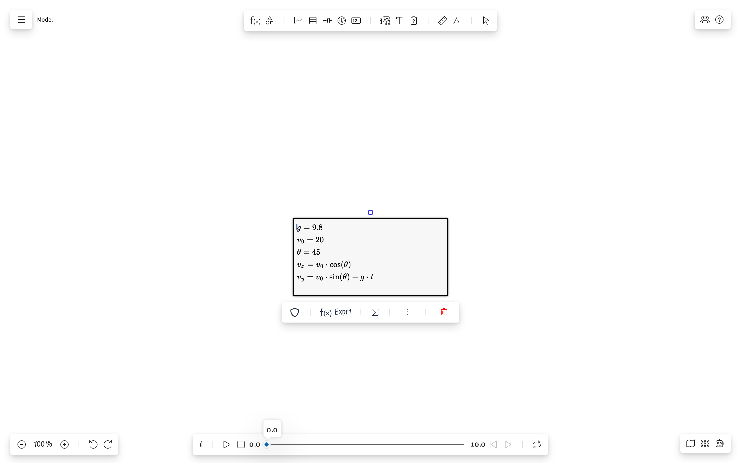
While editing, press ⌘. on macOS or Ctrl+. on Windows/Linux to open the shortcuts palette. You can also open it with the toolbar button.
- Differential equations (dx/dt = ..., shortcut: ⌥ + / on macOS, Alt + / on Windows)
- Recurrences (x_n = x_{n-1} + ...)
- Piecewise functions
- Floor function template
\lfloor x\rfloor - Ceil function template
\lceil x\rceil - Common physics formulas
- Trigonometric identities
Integral Notation
You can enter integral expressions with LaTeX notation such as \int_{a}^{b} f\left(x\right)\,\mathrm{d}x. For integer-part behavior, use the utility function int\left(x\right).
Properties Panel
When an Expression shape is selected, the properties panel shows:
| Property | Description |
|---|---|
| Independent variable | The variable of iteration (default: t) |
| Step | The increment per iteration (Δt) |
| Start / End | Range of the independent variable |
| Initial values | Starting values for differential equations and recurrences |
| Cases | Multiple sets of initial values for parameter studies |
Examples
Simple Kinematics
g = 9.8
v₀ = 20
θ = 45
vx = v₀·\cos\left(θ\right)
vy = v₀·\sin\left(θ\right) - g·t
\frac{dx}{dt} = vx
\frac{dy}{dt} = vy
Population Growth (Recurrence)
r = 0.05
P_{n} = P_{n-1}·\left(1 + r\right)
Piecewise Velocity
v = \begin{cases} 0 & t = 0 \\ a·t & 0 < t < 5 \\ a·5 & \text{otherwise} \end{cases}